Problem Set 6
Recall the Vertex Cover problem from the video lectures: given an undirected graph (with no parallel edges), compute a minimize-size subset of vertices that includes at least one endpoint of every edge. Consider the following greedy algorithm, given a graph \(G\): (1) initialize \(S = \emptyset\); (2) while \(S\) is not a vertex cover of \(G\): (2a) let \(F\) denote the edges with neither endpoint in \(S\); (2b) let \(e\) be some edge of \(F\); (2c) add both endpoints of \(e\) to \(S\); (3) return \(S\).
Consider the following statement: for every graph \(G\) with \(n\) vertices, this greedy algorithm returns a vertex cover with size at most \(f(n)\) times that of an optimal (minimum-size) vertex cover. Which of the following is the smallest choice of the function \(f(n)\) for which this statement is true?
[Hint: suppose the greedy algorithm picks an edge \(e\) with endpoints \(u\) and \(v\). What can you say about every feasible solution to the problem?]
- \(2\)
- \(O(log n)\)
- \(O(\sqrt{n})\)
- \(O(n)\)
ANSWER: What the algorithm finds in the end is a matching (a set of edges no two of which share an endpoint) that is “maximal” (we can’t add any more edges to it and keep it a matching). Note that a “maximum” matching (we cannot do better) is also a “maximal” matching, but the converse is not necessarily true. See the following example:
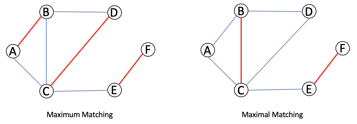
Option 1 is correct. Let \(M\) be a maximal matching, and \(S\) be the set of all endpoints in \(M\).
Claim: The output of the algorithm is feasible.
Proof: We prove this by contradiction: suppose there exists an edge \(e = (u, v)\) such that \(u, v \notin S\). Since \(e\) does not share an endpoint with any of the vertices in \(M\), \(M \cup \{e\}\) is a larger matching, which contradicts \(M\) being a maximal matching.
Lemma: Given algorithm gives a 2-approximation for minimum vertex cover regardless of the choice of \(M\).
Proof: Let \(OPT\) be the minimum vertex cover in graph \(G\). The edges of \(M\) are independent; thus any feasible cover must take at least one vertex from every edge in \(M\). This means that \(\lvert M \rvert \leq OPT\) and then we have:
\[\lvert M \rvert \leq OPT \leq \lvert S \rvert = 2 \lvert M \rvert \leq 2 OPT\]This technique of lower bounding the optimum is often key in proving approximation factors, as we are usually unable to compute the value of OPT.
This algorithm was discovered independently by Fanica Gavril and Mihalis Yannakakis.
In the set cover problem, you are given \(m\) sets \(S_1, \dots, S_m\), each a subset of a common set \(U\) with size \(\lvert U \rvert = n\). The goal is to select as few of these sets as possible, subject to the constraint that the union of the chosen sets is all of \(U\). (You can assume that \(\cup_{i=1}^m S_i = U\).) For example, if the given sets are \(\{1,2\}, \{2,3\}, \text{ and } \{3,4\}\), then the optimal solution consists of the sets \(\{1,2\} \text{ and } \{3,4\}\).
Here is a natural iterative greedy algorithm. First, initialize \(C = \emptyset\), where \(C\) denotes the sets chosen so far. The main loop is: as long as the union \(\cup_{S \in C} S\) of the sets chosen so far is not the entire set \(U\):
- Let \(S_i\) be a set that includes the maximum-possible number of elements not in previously-chosen sets (i.e., that maximizes \(\lvert S_i - \cup_{S \in C} S \rvert\)).
- Add \(S_i\) to \(C\).
Consider the following statement: for every instance of the set cover problem (with \(\lvert U \rvert = n\)), this greedy algorithm returns a set cover with size at most \(f(n)\) times that of an optimal (minimum-size) set cover. Which of the following is the smallest choice of the function \(f(n)\) for which this statement is true?
[Hint: what’s the mininum-possible progress that the greedy algorithm can make in each iteration, as a function of the size of an optimal set cover and of the number of elements that have not yet been covered?]
- \(2\)
- \(O(log n)\)
- \(O(\sqrt{n})\)
- \(O(n)\)
ANSWER: Before giving the proof, we need one useful technical inequality.
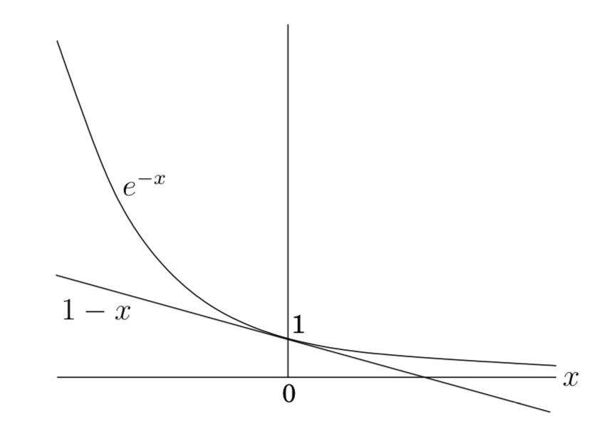
Lemma: For all \(x \gt 0\),
\[(1 - \frac{1}{x})^{x} \leq \frac{1}{x}\]where \(e\) is the base of the natural logarithm.
Proof: We use the fact that for any real \(z\) (positive, zero, or negative), \(1 + z \leq e^z\). (This follows from the Taylor’s expansion \(e^z = 1 + z + \frac{z^2}{2!} + \frac{z^3}{3!} + \dots \geq 1 + z\).) Now, if we substitute \(-\frac{1}{x}\) for \(z\) we have \((1 - \frac{1}{x}) \leq e^{-\frac{1}{x}}\). By raising both sides to the \(x\)th power, we have the desired result. We can also arrive at the same result pictorially as shown below:
We will cheat a bit. Let \(c\) denote the size of the optimum set cover, and let \(g\) denote the size of the greedy set cover minus 1. We will show that \(g \leq c \ln n\). (we could really show that \(g + 1 \leq c \ln n\), but this is close enough and saves us some messy details.)
Let’s consider how many new elements we cover with each round of the algorithm. Initially, there are \(n_0 = n\) elements to be covered. Let \(n_i\) denote the number of elements remaining to be covered after \(i\) iterations of the greedy algorithm. After \(i - 1\) rounds, there are \(n_{i-1}\) elements that remain to be covered. We know that there is a cover of size \(c\) for these elements (namely, the optimal cover), and so by the pigeonhole principal there exists some set that covers at least \(\frac{n_{i−1}}{c}\) elements. Since the greedy algorithm selects the set covering the largest number of remaining elements, it must select a set that covers at least this many elements. The number of elements that remain to be covered is at most
\[n_i \leq n_{i-1} - \frac{n_{i−1}}{c} = n_{i-1}(1 - \frac{1}{c})\]Thus, with each iteration the number of remaining elements decreases by a factor of at least \((1 - \frac{1}{c})\). If we repeat this \(i\) times, we have
\[n_i \leq n_{0}(1 - \frac{1}{c})^i = n(1 - \frac{1}{c})^i\]How long can this go on? Since the greedy heuristic ran for \(g + 1\) iterations, we know that just prior to the last iteration we must have had at least one remaining uncovered element, and so we have
\[1 \leq n_g \leq n(1 - \frac{1}{c})^g = n((1 - \frac{1}{c})^c)^{\frac{g}{c}}\](In the last step, we just rewrote the expression in a manner that makes it easier to apply the above technical lemma.) By the above lemma we have
\[1 \leq n(\frac{1}{e})^{\frac{g}{c}}\]Now, if we multiply by \(e^{\frac{g}{c}}\) on both sides and take natural logs we find that \(g\) satisfies:
\[e^{\frac{g}{c}} \leq n \implies \frac{g}{c} \leq \ln n \implies g \leq c \ln n\]Therefore (ignoring the missing “+1” as mentioned above), the greedy set cover is larger than the optimum set cover by a factor of at most \(\ln n\). Since logs of different bases differ only by a constant factor, option 2 is correct.
Suppose you are given \(m\) sets \(S_1, \dots, S_m\), each a subset of a common set \(U\). The goal is to choose 2 of the \(m\) sets, \(S_i\) and \(S_j\), to maximize the size \(\lvert S_i \cup S_j \rvert\) of their union. One natural heuristic is to use a greedy algorithm: (i) choose the first set \(S_i\) to be as large as possible, breaking ties arbitrarily; (ii) choose the second set \(S_j\) to maximize \(\lvert S_i \cup S_j \rvert\) (i.e., as the set that includes as many elements as possible that are not already in \(S_i\)), again breaking ties arbitrarily. For example, if the given sets are \(\{1,2\}, \{2,3\}, and \{3,4\}\), then the algorithm might pick the set \(\{1,2\}\) in the first step; if it does so, it definitely picks the set \(\{3,4\}\) in the second step (for an objective function value of 4).
Consider the following statement: for every instance of the above problem, the greedy algorithm above chooses two sets \(S_i,S_j\) such that \(\lvert S_i \cup S_j \rvert\) is at least \(c\) times the maximum size of the union of two of the given sets. Which of the following is the largest choice of the constant \(c\) for which this statement is true?
- \(1\)
- \(\frac{1}{2}\)
- \(\frac{2}{3}\)
- \(\frac{3}{4}\)
ANSWER: This is known as the Maximum Coverage Problem. We will prove the lower bound for \(k\) sets, and show that the result doesn’t depend on the number of sets picked. Let \(OPT\) denote the optimal solution; \(x_i\) denote the number of newly covered elements at the \(i\)th iteration; \(y_i\) denote the total number of covered elements up to, and including, the \(i\)th iteration, i.e., \(y_i = \sum_{j=1}^{i} x_i\); and \(z_i\) is the number of uncovered elements after the \(i\)th iteration, i.e., \(z_i = OPT - y_i\). Moreover, \(x_0 = y_0 = 0\), and \(z_0 = OPT\).
Claim 1: \(x{i+1} \geq \frac{z_i}{k}\)
Proof: At each step, the algorithm selects a subset whose inclusion covers the maximum number of uncovered elements. Since the optimal solution uses \(k\) sets to cover \(OPT\) elements, some set must cover at least \(\frac{1}{k}\) fraction of the at least \(z_i\) remaining uncovered elements from \(OPT\). Hence, \(x_{i+1} \geq \frac{z_i}{k}\).
Claim 2: \(z_{i+1} \leq (1 - \frac{1}{k})^{i+1} \cdot OPT\)
Proof: By induction. For \(i = 0, z_1 = (1 - \frac{1}{k}) \cdot OPT\). We assume inductively that \(z_i \leq (1 - \frac{1}{k})^i \cdot OPT\). Then
\[\begin{equation*} \begin{aligned} z_{i+1} & \leq z_i - x_{i+1} \\ & \leq z_i(1 - \frac{1}{k}) && \text{-- using Claim 1} \\ & \leq (1 - \frac{1}{k})^{i+1} \cdot OPT && \text{-- using the inductive hypothesis} \end{aligned} \end{equation*}\]Lemma: The algorithm is a \(1 - \frac{1}{e}\) approximation for the optimal solution.
Proof: Using Claim 2, and the fact that \((1 - \frac{1}{k}) \leq e^{-\frac{1}{k}}\) (shown earlier), we have \(z_k \leq (1 - \frac{1}{k})^k \cdot OPT \leq \frac{OPT}{e}\). Hence, \(y_k = OPT - z_k \geq (1 - \frac{1}{e}) \cdot OPT\).
Lastly, since \(\frac{1}{e} \approx 0.37, 1 - \frac{1}{e} \approx 0.63\). Option 3 is right, since \(\frac{2}{3} \approx 0.67\), the closest to \(1 - \frac{1}{e}\).
Consider the following job scheduling problem. There are \(m\) machines, all identical. There are \(n\) jobs, and job \(j\) has size \(p_j\). Each job must be assigned to exactly one machine. The load of a machine is the sum of the sizes of the jobs that get assigned to it. The makespan of an assignment of jobs is the maximum load of a machine; this is the quantity that we want to minimize. For example, suppose there are two machines and \(4\) jobs with sizes \(7,8,5,6\). Assigning the first two jobs to the first machine and the last two jobs to the second machine yields machine loads \(15\) and \(11\), for a makespan of \(15\). A better assignment puts the first and last jobs on the first machine and the second and third jobs on the second machine, for a makespan of \(13\).
Consider the following greedy algorithm. Iterate through the jobs \(j = 1,2,3,\dots,n\) one-by-one. When considering job \(j\), assign it to the machine that currently has the smallest load (breaking ties arbitrarily). For example, in the four-job instance above, this algorithm would assign the first job to the first machine, the second job to the second machine, the third job to the first machine, and the fourth job to the second machine (for a suboptimal makespan of \(14\)).
Consider the following statement: for every such job scheduling instance, this greedy algorithm computes a job assignment with makespan at most \(c\) times that of an optimal (minimum-makespan) job assignment. Which of the following is the smallest choice of the constant \(c\) that makes this statement true?
[Hint: let \(A\) and \(B\) denote the average and maximum job sizes \((A = \frac{\sum_j p_j}{m}\) and \(B = \max_j p_j\)). Try to relate both the optimal solution and the output of the greedy algorithm to \(A, B\).]
- \(2\)
- \(\frac{6}{5}\)
- \(\frac{3}{2}\)
- \(4\)
ANSWER: Let \(P^*\) be the optional solution, One of the lower bounds on \(P^*\) is given by \(A\), because clearly, we can’t do better than assigning every machine the same load.
Lemma 1: \(P^* \geq A\)
However, there is one case where this lower bound is too weak to be useful; when the size of one job dominates all the other. Thus, an additional lower bound is given by Lemma 2.
Lemma 2: \(P^* \geq B\)
Consider machine \(M_i\) that attains the maximum load in our assignment. Let \(P_i\) be the load after the assignment of job \(j\) to it. Just before job \(j\) was assigned to \(M_i\), the load on it was the smallest of any machine; therefore, every machine had a load of at least \(P_i - p_j\). Adding up the loads of all machines at that point, we have
\[\begin{equation*} \begin{aligned} m(P_i - p_j) & \leq \sum_{k=1}^{m} p_j \\ (P_i - p_j) & \leq \frac{1}{m} \sum_{k=1}^{m} p_j \\ (P_i - p_j) & \leq A \\ (P_i - p_j) & \leq P^* && \text{-- using Lemma 1} \end{aligned} \end{equation*}\]\(p_j\) can at most be \(B\); i.e. \(p_j \leq B \implies P^* \geq p_j\) (using Lemma 2). After assigning job \(j\) to machine \(M_i\), its load is given by \(P_i - p_j + p_j \leq 2P^*\). Therefore, the greedy algorithm is a 2-approximation algorithm, and option 1 is correct.
Consider the same makespan-minimization job scheduling problem studied in the previous problem. Now suppose that, prior to running the greedy algorithm in the previous problem, we first sort the jobs from biggest to smallest. For example, in the four-job instance discussed in the previous problem, the jobs would be considered in the order \(8,7,6,5\), and the greedy algorithm would then produce an optimal schedule, with makespan \(13\).
Consider the following statement: for every such job scheduling instance, the greedy algorithm (with this sorting preprocessing step) computes a job assignment with makespan at most \(c\) times that of an optimal (minimum-makespan) job assignment. Which of the following is the smallest choice of the constant \(c\) for which this statement is true?
- \(\frac{3}{2}\)
- \(2\)
- \(\frac{6}{5}\)
- \(4\)
ANSWER:
Lemma: If there are more than \(m\) jobs, \(P^* \geq 2p_{m+1}\)
Proof: If there are as many jobs as there are machines, then the optimal assignment is trivial; every machine gets a job. The optimal makespan is \(B\). When there are more than \(m\) jobs, since they are assigned in decreasing order of size, size of job \(m + 1\) is no bigger than that of any of the jobs \(1\) through \(m\). Since there are \(m\) machines, and at least \(m + 1\) jobs, by the Piegeonhole Principle, one machine is assigned two jobs, and its load is at least \(2p_{m+1}\).
As before, we consider a machine \(M_i\) that has the maximum load. If \(M_i\) only holds a single job, then the schedule is optimal. So let’s assume that machine \(M_i\) has at least two jobs, and let \(p_j\) be the size of the last job assigned to the machine. Note that \(j \geq m + 1\), since the algorithm will assign the first \(m\) jobs to \(m\) distinct machines. Thus \(p_j \leq p_{m+1} \leq \frac{1}{2}P^*\) (by the Lemma above).
The rest of the proof is very similar to that of the previous one. \(P_i - p_j + p_j \leq P^* + \frac{1}{2}P^* = \frac{3}{2}P^*\). Thus, option 1 is correct.
Which of the following statements is NOT true about the generic local search algorithm?
- The generic local search algorithm is guaranteed to eventually converge to an optimal solution.
- The output of the generic local search algorithm generally depends on the choice of the starting point.
- The output of the generic local search algorithm generally depends on the choice of the superior neighboring solution to move to next (in an iteration where there are multiple such solutions).
- In some cases, the generic local search algorithm can require an exponential number of iterations before terminating.
ANSWER: Option 1 is false. Local search is guaranteed to eventually converge to an locally optimal solution, which at times, can be quite far from a globally optimal solution.
Options 2, 3 and 4 is correct; see lecture video 18.4.
Suppose we apply local search to the minimum cut problem. Given an undirected graph, we begin with an arbitrary cut (A,B). We check if there is a vertex v such that switching v from one group to the other would strictly decrease the number of edges crossing the cut. (Also, we disallow vertex switches that would cause A or B to become empty.) If there is such a vertex, we switch it from one group to the other; if there are many such vertices, we pick one arbitrarily to switch. If there are no such vertices, then we return the current locally optimal cut (A,B). Which of the following statements is true about this local search algorithm?
- This local search algorithm is guaranteed to terminate in a polynomial number of iterations.
- This local search algorithm is guaranteed to compute a minimum cut.
- This local search algorithm is guaranteed to compute a cut for which the number of crossing edges is at most twice the minimum possible.
- If this local search algorithm is guaranteed to terminate in a polynomial number of iterations, it would immediately imply P = NP.
ANSWER: Option 1 is true. Every iteration strictly decreases the number of crossing edges, so there can be only \(m\) iterations.
Options 2 and 3 are false.
Option 4 is false. local search is guaranteed to eventually converge to an locally optimal solution, whereas P = NP implies we can find a globally optimal solution in polynomial time.
In the maximum \(k\)-cut problem, the input is an undirected graph \(G = (V, E)\), and each edge has a nonnegative weight \(w_e\). The goal is to partition \(V\) into \(k\) non-empty pieces \(A_1,\dots,A_K\) to maximize the total weight of the cut edges (i.e., edges with endpoints in different \(A_i\)’s). The maximum cut problem (as studied in lecture) corresponds to the special case where \(k = 2\).
Consider applying local search to the maximum \(k\)-cut problem: (i) start with an arbitrary \(k\)-cut; (ii) repeat: if possible, move a vertex from one set \(A_i\) to another set \(A_j\) so as to strictly increase the total weight of the cut edges; (iii) once no such move is possible, halt.
Consider the following statement: for every instance of the maximum \(k\)-cut problem, every local maximum has objective function value at least \(f(k)\) times that of the maximum possible. Which of the following is the biggest choice of the function \(f(k)\) for which this statement is true?
- \(\frac{1}{2}\)
- \(1 - \frac{1}{k(k - 1)}\)
- \(\frac{1}{k}\)
- \(\frac{k - 1}{k}\)
ANSWER: This paper presents a local search solution that achieves a lower bound no smaller than \(1 - \frac{1}{k}\) of the optimal solution. It appears that none of the given options are correct.
Suppose \(X\) is a random variable that has expected value \(1\). What is the probability that \(X\) is \(2\) or larger? (Choose the strongest statement that is guaranteed to be true.)
- At most \(100\%\)
- At most \(25\%\)
- \(0\)
- At most \(50\%\)
ANSWER: Consider the following probability distribution for \(X\):
\[P(X) = \begin{cases} 0.9 \text{ if } X = 2 \\ 0.1 \text{ if } X = -1 \\ 0 \text{ otherwise} \end{cases}\]Then \(E(X) = 1\) yet \(P(X \geq 2) = 0.9\). This counterexample eliminates the second, third, and fourth options. So, option 1 is correct.
Suppose \(X\) is a random variable that is always nonnegative and has expected value \(1\). What is the probability that \(X\) is \(2\) or larger? (Choose the strongest statement that is guaranteed to be true.)
- At most \(100\%\)
- At most \(25\%\)
- \(0\)
- At most \(50\%\)
ANSWER: Using Markov’s Inequality, we have:
\[\begin{equation*} \begin{aligned} P(X \geq 2) & \leq \frac{E[X]}{2} \\ & = \frac{1}{2} \end{aligned} \end{equation*}\]Therefore, option 4 is correct.

Comments